A vector space (also called a linear space) consists of:

• A set of vectors: $\psi,\phi,\chi ,\cdots$,
• A set of scalars: $a,b,c,\cdots$ (these will always be real or complex numbers in quantum mechanics),
• A rule for the addition of vectors: $\psi + \phi$,
• A rule for multiplying vectors by scalars: $a \psi$.

The addition rule is required to make the set of vectors into an abelian group. For the uninitiated, this means:

• If $\psi$ and $\phi$ are vectors, then $\psi + \phi$ is also a vector.
• Commutativity: $\psi + \phi = \phi + \psi$,
• Associativity: $(\psi + \phi) + \chi = \psi + (\phi + \chi)$,
• There exists a vector $\boldsymbol{0}$ such that, for all vectors $\psi$, \[\boldsymbol{0} + \psi = \psi + \boldsymbol{0} = \psi,\]
• For each vector $\psi$, there exists a unique vector $-\psi$ such that \[\psi + (-\psi) = (-\psi) + \psi = \boldsymbol{0}.\]

The scalar multiplication rule must satisfy:

• For every scalar $a$ and vector $\psi$, $a\psi$ is a vector.

  • Taken together with the addition rule, this means that $a\psi + b\phi$ is always a vector for any scalars $a,b$ and vectors $\psi,\phi$. In other words, we can take linear combinations of vectors.
• Distributivity: $a(\psi + \phi) = a\psi + a \phi$ and $(a+b)\psi = a\psi + b\psi$.
• Associativity: $a(b\psi) = (ab)\psi$.
• There exists a unit scalar $1$ and a zero scalar $0$ such that, for all vectors $\psi$, \[1\psi = \psi,\qquad\qquad 0\psi = \boldsymbol{0}.\]

  • Note: in the second equation, it is the zero scalar on the left hand side and the zero vector on the right hand side.

• $\mathbb{R}^n$: The set of $n$-dimensional column vectors with real components.

  • Addition is component-wise addition.
  • Scalars are the real numbers. \[\vec{r} = \left ( \begin{array}{r} r_1 \\ r_2 \\ \vdots \\ r_n \end{array} \right )\]

• $\mathbb{C}^n$: The set of $n$-dimensional column vectors with complex components.

  • Addition is component-wise addition.
  • Scalars are the complex numbers. \[\vec{z} = \left ( \begin{array}{r} z_1 \\ z_2 \\ \vdots \\ z_n \end{array} \right )\]
• $\mathbb{C}^{\infty}$: The set of $\infty$-dimensional column vectors with complex components.

• The set of complex-valued functions of a real number $x$.

  • Addition is $(\psi + \phi)(x) = \psi(x) + \phi(x)$.
  • Scalars are the complex numbers with $(z\psi)(x) = z\psi(x)$.

A set of $N$ nonzero vectors $\phi_1,\phi_2,\cdots,\phi_N$ is linearly independent iff the only solution to the equation \[\sum_{n=1}^N a_n \phi_n = 0,\] is \[a_1 = a_2 = \cdots = a_N = 0.\]

Otherwise, the vectors are linearly dependent, and any one of the vectors can be written as a sum of the others, e.g. \[\phi_j = \sum_{n=1}^{j-1} b_n \phi_n + \sum_{n=j+1}^N b_n,\] with $b_n = -a_n/a_j$.

The dimension $d$ of a vector space is the maximum number of linearly independent vectors that exist in the space.

A basis $\phi_1,\phi_2,\cdots,\phi_d$ for a vector space of dimension $d$ is a set of linearly independent vectors of maximal size. This implies that, for a basis, all vectors can be written as \[\psi = \sum_{n=1}^d b_n \phi_n,\] for some components $b_n$.

• For $\mathbb{R}^n$ and $\mathbb{C}^n$, the vectors $\vec{e}_j = \left ( \begin{array}{c} 0 \\ \vdots \\ 0 \\ 1 \\ 0 \\ \vdots \\ 0 \end{array} \right )$, where the $j^{\text{th}}$ component is $1$ and all other components are $0$, are a basis (but not the only one).

• For example, for $\mathbb{R}^2$ and $\mathbb{C}^2$, $\left ( \begin{array}{c} 1 \\ 0 \end{array} \right ), \left ( \begin{array}{c} 1 \\ 1 \end{array} \right )$ is also a basis.

• $\mathbb{R}^n$ and $\mathbb{C}^n$ have dimension $n$.

• $\mathbb{C}^{\infty}$ has dimension (countable) infinity.

• The space of complex functions of a real variable has dimension (uncountable) infinity.

A subspace $V'$ of a vector space $V$ is a subset of the vectors that is itself a vector space, i.e. it is closed under taking linear combinations of vectors. The fact that $V'$ is a subspace of $V$ is denoted $V' \subset V$. Clearly, the dimension of a subspace of $V$ is less than or equal to the dimension of $V$.

For example $\mathbb{R}^n \subset \mathbb{C}^n$ consisting of those vectors that only have real components. If we take a linear combination $a\psi + b\phi$ of such vectors with real numbers $a$ and $b$ (which are the scalars of $\mathbb{R}^n$) then it will also be a vector in $\mathbb{R}^n$.

This is an example where the scalars of the subspace are different from the scalars of the original space. However, the most relevant examples for our purposes are where the scalars of the subspace and original space are the same. An example is that $\mathbb{C}^m \subset \mathbb{C}^n$ for $m\leq n$. For a concrete example, consider $\mathbb{C}^3$. The set of vectors of the form \[\left ( \begin{array}{c} a \\ b \\ 0 \end{array} \right ),\] where $a$ and $b$ are complex numbers is a two-dimensional subspace of $\mathbb{C}^3$, as taking linear combinations of such vectors will not change the zero in the third component. You can see that it is two-dimensional by noting that \[\left ( \begin{array}{c} 1 \\ 0 \\ 0\end{array}\right ),\qquad \left ( \begin{array}{c} 0 \\ 1 \\ 0 \end{array}\right ),\] is a basis for it.

This subspace is effectively the same as $\mathbb{C}^2$. If we do not bother to write down the third component then we do have a vector in $\mathbb{C}^2$ and we can always reconstruct the vector in $\mathbb{C}^3$ that it came from by just putting the zero back in the third component. Mathematicians would say that $\mathbb{C}^2$ is isomorphic to this subspace of $\mathbb{C}^3$, which means that there exists a one-to-one map between vectors in the subspace and vectors in $\mathbb{C}^3$.

The distinction is somewhat important because $\mathbb{C}^2$ can be embedded in $\mathbb{C}^3$ in a variety of different ways. For example, The set of all vectors of the form \[\left ( \begin{array}{c} a \\ b \\ 0 \end{array} \right ),\] the set of all vectors of the form \[\left ( \begin{array}{c} a \\ 0 \\ b \end{array} \right ),\] and the set of all vectors of the form \[\left ( \begin{array}{c} 0 \\ a \\ b \end{array} \right ),\] are all two-dimensional subspaces of $\mathbb{C}^3$ that are isomorphic to $\mathbb{C}^2$, but they are different subspaces of $\mathbb{C}^3$.

These examples, are pretty trivial. For a less trivial example, note that the set of all vectors of the form \[\left ( \begin{array}{c} a \\ a \\ b\end{array}\right ),\] is also a two-dimensional subspace of $\mathbb{C}^3$ that is isomorphic to $\mathbb{C}^2$. One possible basis for this subspace is \[\left ( \begin{array}{c} 1 \\ 1 \\ 0\end{array}\right ),\qquad \left ( \begin{array}{c} 0 \\ 0 \\ 1\end{array}\right ).\]

For any vector space, consider the set of linear functions from vectors to scalars. Such a function $f$ assigns a scalar $f(\psi)$ to every vector $\psi$ and satisfies \[f(a\psi + b\phi) = af(\psi) + bf(\phi).\]

If we define the addition and multiplication for such functions via \[(f+g)(\psi) = f(\psi) + g(\psi),\] and \[(af)(\psi) = f(a^* \psi),\] then the set of such functions is also a vector space called the dual vector space. A function $f$ in this space is called a dual vector.

Note that physicists use $^*$ to denote a complex conjugate.

An inner product on a vector space is a function $(\phi,\psi)$ from pairs of vectors to scalars that satisfies:

• Conjugate symmetry: $(\psi,\phi) = (\phi,\psi)^*$.
• Linearity: $(\chi, a\psi + b\phi) = a(\chi,\psi) + b(\chi,\phi)$.
• Positive definiteness: $(\psi,\psi) \geq 0 \qquad$ and $\qquad (\psi,\psi) = 0\,\, \Rightarrow\,\, \psi = \boldsymbol{0}.$

Note that mathematicians usually define inner products to be linear in the first argument. In physics we always define them to be linear in the second argument.

An inner product space is a vector space equipped with an inner product.

Two vectors $\psi$ and $\phi$ in an inner product space are called orthogonal if $(\phi,\psi) = 0$.

• For $\mathbb{R}^n$ and $\mathbb{C}^n$, the dot product is an inner product.

  • $\mathbb{R}^n$: $\left ( \begin{array}{c} r_1 \\ r_2 \\ \vdots \\ r_n \end{array} \right ) \cdot \left ( \begin{array}{c} r_1' \\ r_2' \\ \vdots \\ r_n' \end{array}\right ) = r_1r_1' + r_2 r_2' + \cdots + r_nr_n'$
  • $\mathbb{C}^n$: $\left ( \begin{array}{c} z_1 \\ z_2 \\ \vdots \\ z_n \end{array} \right ) \cdot \left ( \begin{array}{c} z_1' \\ z_2' \\ \vdots \\ z_n' \end{array} \right ) = z_1^*z_1' + z_2^* z_2' + \cdots + z_n^*z_n'$

An inner product induces a one-to-one map between vectors and dual vectors, constructed as follows:

• Given a vector $\phi$, the map $f_{\phi}$ where $f_{\phi}(\psi) = (\phi,\psi)$ is a linear map from vectors to scalars, so it is a dual vector.\
• Firther any linear map from vectors to scalars can be written as $f_{\phi}$ for some vector $\phi$. (Proving this for $\mathbb{R}^n$ is an in class activity.)

In $\mathbb{R}^n$ and $\mathbb{C}^n$ we usually think of the dual vectors as row vectors, and then the action of a dual vector on a vector becomes matrix multiplication, i.e. in $\mathbb{C}^n$ for a vector \[\vec{s} = \left ( \begin{array}{r} s_1 \\ s_2 \\ \vdots \\ s_n \end{array}\right ),\] we define \[\boldsymbol{f}_{\vec{s}} = ( s_1^*,s_2^*,\cdots,s_n^*),\] and then, for any other vector $\vec{z}$, we have \[f_{\vec{s}}(\vec{z}) = \vec{s} \cdot \vec{z} = \boldsymbol{f}_{\vec{s}}\vec{z},\] where $\boldsymbol{f}_{\vec{s}}\vec{r}$ is just matrix multiplication of the row vector $\boldsymbol{f}_{\vec{s}}$ with the column vector $\vec{z}$.

A basis $\phi_1,\phi_2,\cdots,\phi_d$ for a $d$-dimensional inner product space is called orthonormal if \[(\phi_j,\phi_k) = \delta_{jk} = \begin{cases} 0, & j\neq k \\ 1, & j=k\end{cases}\]

For any basis, we can write any vector as $\psi = \sum_{j=1}^d b_j \phi_j$, and if the basis is also orthonormal then \[(\phi_k,\psi) = \sum_{j=1}^d b_j (\phi_k,\phi_j) = \sum_{j=1}^d b_j \delta_{jk} = b_k,\] so there is an easy way of finding the components of a vector in an orthonormal basis by just taking the inner products \[b_k = (\phi_k,\psi).\] Note: this only works in an orthonormal basis.

As an example, in $\mathbb{R}^2$ and $\mathbb{C}^d$, the basis $\left ( \begin{array}{c} 1 \\ 0 \end{array} \right ), \left ( \begin{array}{c} 0 \\ 1 \end{array} \right )$ is orthonormal but the basis $\left ( \begin{array}{c} 1 \\ 0 \end{array} \right ), \left ( \begin{array}{c} 1 \\ 1 \end{array} \right )$ is not.

In an inner product space, subspaces have more structure. Suppose that $V_1 \subset V$ and $V_2 \subset V$. $V_1$ and $V_2$ are orthogonal subspaces of $V$ if $(\psi,\phi) = 0$ for all vectors $\psi \in V_1$ and $\phi \in V_2$. As an example, the set of all vectors of the form \[\left ( \begin{array}{c} a \\ 0 \\ 0 \end{array}\right ),\] and the set of all vectors of the form \[\left ( \begin{array}{c} 0 \\ a \\ 0 \end{array}\right ),\] are orthogonal subspaces of $\mathbb{C}^3$. For a less trivial example, the set of all vectors of the form \[\left ( \begin{array}{C} a \\ a \\ b \end{array}\right ),\] and the set of vectors of the form \[\left ( \begin{array}{c} a \\ -a \\ 0 \end{array} \right ),\] are orthogonal subspaces of $\mathbb{C}^3$

Suppose $V' \subset V$. Then, we can construct another subspace $V'^{\perp}$ called the orthogonal complement of $V'$ in $V$. It consists of all vectors $\phi$ such that, for all vectors $\psi \in V'$, $(\psi,\phi) = 0$.

It is easy to see that this is indeed a subspace. If $\phi, \chi \in V'^{\perp}$ and $\psi \in V'$ then, for any scalars $a$ and $b$ \[(\psi,a\phi + b\chi) = a(\psi,\phi) + b(\psi,\chi) = a\times 0 + b\times 0 = 0,\] i.e. the orthogonality property is preserved under taking linear combinations, due to the linearity of the inner product in its second argument.

A set of orthogonal subspaces $V_1,V_2,\cdots \subset V$ is said to span the inner product space $V$ if all vectors $\psi \in V$ can be written as \[\psi = \sum_j \psi_j,\] where $\psi_j \in V_j$. We sometimes write this as $V = \oplus_j V_j$

As an example, let $\phi_1,\phi_2,\cdots$ be an orthonormal basis for $V$ and let $V_j$ be the one dimensional subspace consisting of all vectors of the form $a\phi_j$. Then, $V = \oplus_j V_j$ just by the definition of a basis, i.e. all vectors $\psi \in V$ can be written as \[\psi = \sum_j a_j \phi_j.\]

As a less trivial example, for any subspace $V' \subset V$, we have $V = V' \oplus V'^{\perp}$. To see this, note that if $\phi_1,\phi_2,\cdots$ is an orthonormal basis for $V'$ and $\chi_1,\chi_2,\cdots$ is an orthonormal basis for $V'^{\perp}$ then $\phi_1,\phi_2,\cdots,\chi_1,\chi_2,\cdots$ is a basis for $V$. Any vector $\psi$ can be written in this basis as \[\psi = \sum_j a_j \phi_j + \sum_k b_k \chi_k,\] and then if we define \begin{align*} \psi' & = \sum_j a_j \phi_j, & \psi'^{\perp} & = \sum_k b_k \chi_k, \end{align*} we have \[\psi = \psi' + \psi'^{\perp},\] where $\psi' \in V'$ and $\psi'^{\perp} \in V'^{\perp}$.

On an inner product space, we define the norm of a vector as \[||\psi|| = \sqrt{(\psi,\psi)}.\] In $\mathbb{R}^n$ the norm is just the length of the vector $\sqrt{r_1^2 + r_2^2 +\cdots+r_n^2}$.

The norm satisfies the following properties

• $||\psi|| \geq 0$ for all vectors $\psi$.
• $||\psi|| = 0$ if and only if $\psi = \boldsymbol{0}$.
• $||a\psi|| = |a| ||\psi||$ for all scalars $a$ and vectors $\psi$.

These properties follow directly from the properties of inner products and the definition of the norm.

The Cauchy-Schwartz inequality states that: \[|(\phi,\psi)| \leq ||\psi|| ||\phi||.\]

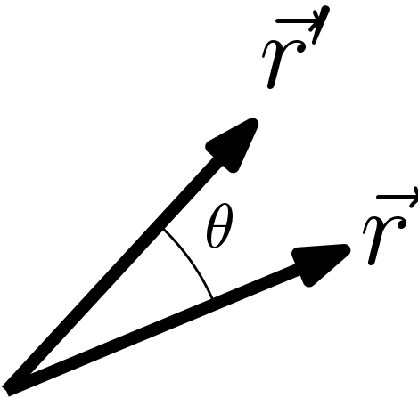
To understand the meaning of this, it is helpful to recall the geometric interpretation of the inner product (dot product) in $\mathbb{R}^2$. If we have two vectors $\vec{r}$ and $\vec{r}'$ then $\vec{r}\cdot \vec{r}' = ||\vec{r}|| ||\vec{r}'|| \cos \theta$, where $||\vec{r}||$ and $||\vec{r}'||$ are the lengths of the vectors $\vec{r}$ and $\vec{r}'$, and $\theta$ is the angle between them. This is illustrated below.

Since $-1 \leq \cos\theta \leq 1$, we obviously have \[|\vec{r}\cdot \vec{r}'| \leq ||\vec{r}|| ||\vec{r}'||,\] which is the special case of the Cauchy-Schwartz inequality for $\mathbb{R}^2$.

A useful special case of the Cauchy-Schwartz inequality is when $\psi$ and $\phi$ are unit vectors, i.e. $||\psi|| = ||\phi|| = 1$. This is the usual case in quantum mechanics because we usually normalize our wavefunctions. In this case, the Cauchy-Schwartz inequality says that $|(\phi,\psi)| < 1$. This will be used to prove that the probability rule in quantum mechanics gives well-defined probabilities.

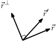
To prove the Cauchy-Schwartz inequality in full generality, we start from the observation that, for any two vectors $\psi$ and $\phi$, we can always write \[\phi = a \psi + b\psi^{\perp},\] where $a$ and $b$ are scalars, and $\psi^{\perp}$ is orthogonal to $\psi$, i.e. $(\psi^{\perp},\psi) = 0$.

Proving that this is the case, and then proving the Cauchy-Schwartz inequality from it, is an in class activity. However, to aid intuition, consider again the case of $\mathbb{R}^2$. Any two vectors, $\vec{r}$ and $\vec{r}'$ form a basis, provided they are linearly independent. It is then possible to find an orthogonal vector $\vec{r}^{\perp}$, such that $\vec{r}$ and $\vec{r}^{\perp}$ are orthogonal and also form a basis. Therefore, it is possible to write $\vec{r}'$ as a linear combination of $\vec{r}$ and $\vec{r}^{\perp}$. This is illustrated below.

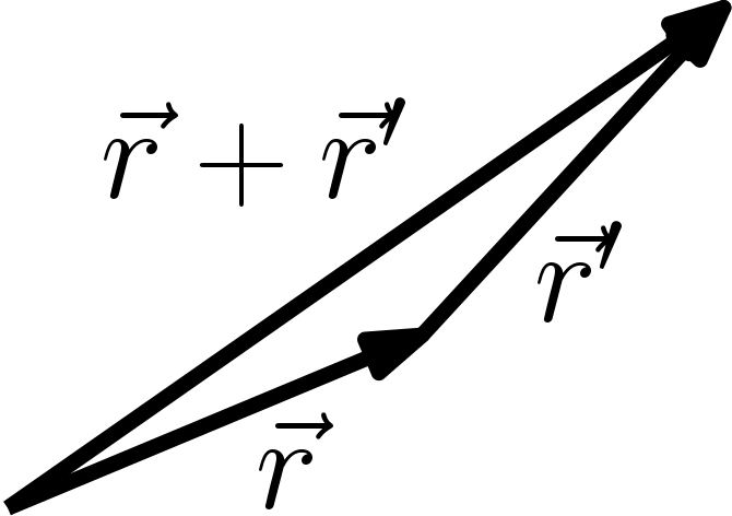
The triangle inequality states that \[||\psi + \phi || \leq ||\psi|| + ||\phi||.\] It is called the triangle inequality because, in the special case of $\mathbb{R}^2$, it says that the sum of the lengths of two sides of a triangle is greater than or equal to the length of the third, as illustrated below.

In general, we can use the Cauchy-Schwartz inequality to prove the triangle inequality as follows. \begin{align*} ||\psi + \phi ||^2 & = (\psi + \phi,\psi + \phi) & \text{by the definition of the norm} \\ & = (\psi,\psi) + (\phi,\psi) + (\psi,\phi) + (\phi,\phi) & \text{by linearity} \\ & = ||\psi||^2 + 2\text{Re}(\phi,\psi) + ||\phi||^2 & \text{by the definition of the norm and conjugate symmetry} \\ & \leq ||\psi||^2 + 2|(\phi,\psi)| + ||\phi||^2, \end{align*} where the last line follows because, for a complex number $z$, $|z| = \sqrt{\text{Re}(z)^2 + \text{Im}(z)^2} \geq \text{Re}(z)$.

We can now apply the Cauchy-Schwartz inequality $|(\phi,\psi)| \leq ||\psi|| ||\phi||$ to obtain \begin{align*} ||\psi + \phi ||^2 & = \leq ||\psi||^2 + 2||\psi|| ||\phi|| + ||\phi||^2 \\ & = \left ( ||\psi|| + ||\phi||\right )^2, \end{align*} from which the triangle inequality follows by taking the square root.

From the point of view of this course, a Hilbert space is an inner product space that might be finite or infinite-dimensional, but if it is infinite dimensional then it is well-behaved enough to have all the properties of a finite-dimensional space that we need to get things to work nicely. In other words, in this course, we will often only prove things for the finite dimensional case and then just assume that they are true in infinite dimensions as well. Although this is not the case for a general infinite dimensional inner product space, it is true if we invoke the magic words of mathematical gobbledygook “Hilbert Space”.

For those of you who are interested in the details, a Hilbert space $\mathcal{H}$ is a complete inner product space. This means that every Cauchy sequence of vectors $\psi_n \in \mathcal{H}$ converges to a vector in $\mathcal{H}$. What is a Cauchy sequence you ask? It is a sequence of vectors $\psi_n \in \mathcal{H}$ such that $\lim_{m,n\rightarrow \infty}||\psi_n - \psi_m|| = 0$, so in a Hilbert space, whenever $\lim_{m,n\rightarrow \infty}||\psi_n - \psi_m|| = 0$ for a sequence of vectors then there is a unique vector $\psi \in \mathcal{H}$ such that $\lim_{n\rightarrow \infty} \psi_n = \psi$.

The Hilbert spaces that we deal with in quantum mechanics are usually seperable. This means that there exists a Cauchy sequence $\psi_n$ such that, for every vector $\psi$ and every $\epsilon > 0$, there exists at least one $\psi_n$ such that $||\psi - \psi_n || < \epsilon$.

I do not expect you to understand any of this. The mathematically inclined can look up the details in a textbook on functional analysis or a book on quantum mechanics aimed at mathematicians. The point is just to note that there is rigorous mathematics behind some of the non-rigorous leaps we will take in this course. Hilbert spaces are defined such that, if they are infinite dimensional, they still have properties similar to $\mathbb{R}^n$ and $\mathbb{C}^n$. We shall not worry about the technical details too much, but rather assume, like good physicists, that things we can prove in $\mathbb{C}^n$ also hold in the infinite dimensional Hilbert spaces of quantum mechanics.

Seperable Hilbert spaces always have a countable basis (in fact, this is equivalent to seperability). This is usually true in quantum mechanics, e.g. the discrete energy states of a hydrogen atom.

The Hilbert space that we will be working with most often in this course is the space of square integrable functions. Consider the space of complex functions of a real variable. We can define an inner product on this space via \[(\phi,\psi) = \int_{-\infty}^{+\infty} \phi^*(x)\psi(x)\,\mathrm{d}x.\] Technically, in order to make this into an inner product space, we need to identify functions that differ on sets of measure zero and make the vectors the equivalence classes of such functions.

In this inner product space, the inner products and norms can be infinite, e.g. consider $||\psi|| = \sqrt{(\psi,\psi)}$ when $\psi(x) = c$ for some constant $c$. Then \[(\psi,\psi) = \int_{-\infty}^{+\infty}c^2 \,\mathrm{d}x = \infty.\] Since the Born rule in quantum mechanics tells us that integrals of the form $\int |\psi(x)|^2$ have to do with probabilities, we want to ensure that $(\psi,\psi) = \int_{-\infty}^{+\infty} |\psi(x)|^2$ is always finite. Therefore, the Hilbert space of square integrable functions is defined to be the set of functions $\psi(x)$ such that \[||\psi||^2 = (\psi,\psi) = \int_{-\infty}^{+\infty} |\psi(x)|^2,\] is finite.

Note that, by the Cauchy-Schwartz inequality, the inner product $(\psi,\phi) = \int_{-\infty}^{+\infty} \phi^*(x)\psi(x)\,\mathrm{d}x$ is always finite in this Hilbert space because $|(\psi,\phi)|\leq ||\psi|| ||\phi||| < \infty$.

In quantum mechanics, we normally work with normalized wavefunctions, so that \[||\psi||^2 = \int_{-\infty}^{+\infty} |\psi(x)|^2 = 1,\] rather than just being finite. However, it is convenient to also include scalar multiples of these functions, i.e. unnormalized wavefunctions, in the space that we are working with so that it is a vector space.

1. Prove that an inner product satisfies conjugate linearity, i.e. \[(a\psi + b\phi,\chi) = a^*(\psi,\chi) + b^*(\phi,\chi).\] For the space of complex functions of a real variable $x$, why isn't \[(\phi,\psi) = \int_{-\infty}^{+\infty} \phi^*(x)\psi(x)\,\mathrm{d}x,\] an inner product?
2. For the vector space $\mathbb{R}^n$, prove that any linear map $f$ from vectors to scalars can be written as \[f(\vec{r}) = \vec{s}\cdot\vec{r},\] for some vector $\vec{s}$. HINT: Consider how $f$ acts on the basis vectors \[\vec{e}_j = \left ( \begin{array}{c} 0 \\ \vdots \\ 0 \\ 1 \\ 0 \\ \vdots \\ 0 \end{array} \right ),\] where the $j^{\text{th}}$ component is $1$ and all other components are $0$.
3. For two vectors $\psi$ and $\phi$, prove that the vector \[\psi^{\perp} = (\psi,\psi)\phi - (\psi,\phi)\psi,\] is orthogonal to $\psi$ and that \[\phi = a\psi + b\psi^{\perp},\] for some scalars $a$ and $b$, what are the values of $a$ and $b$? By taking the inner product of this equation with $\phi$, prove the Cauchy-Schwartz inequality.