A wavefunction of the form $\psi(x,t) \propto e^{i(kx - \omega t)}$ has a well-defined momentum, but is spread out over all space. See the graph below for an illustration of what this wavefunction looks like for $k = \pi$, $t=0$.

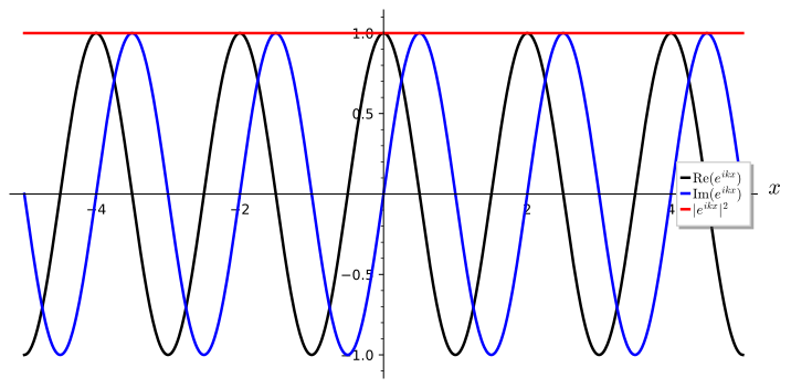
The wavefunction $\psi(x,t) \propto e^{i(kx - \omega t)}$ is also not normalizable because \[\int_{-\infty}^{+\infty} |\psi(x)|^2\,\mathrm{d}x = \int_{-\infty}^{+\infty} \,\mathrm{d}x = \infty,\] so it does not give us a well-defined probability distribution. Therefore, it cannot be a physically realizable wavefunction.

Similarly, if we want to describe a particle with a well-defined position $x = x_0$, we would use $\psi(x,t) = \delta(x-x_0)$, where $\delta(x - x_0)$ is a Dirac delta function. These will be defined more rigorously in the next module, but for now you can think of it as a “function” that is zero everywhere except at $x=x_0$, where it suddenly jumps to infinity. The Dirac delta function $\delta(x-2)$ is illustrated below.

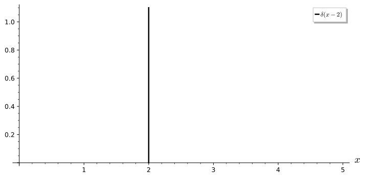
By the uncertainty principle, since $\Delta x = 0$, we must have $\Delta p =\hbar/2\Delta x = \infty$, so these wavefunctions are spread out over all possible momenta. Dirac delta functions are also not normalizable, so again they cannot be physically realizable wavefunctions.

In fact, we will use these kinds of wavefunctions to solve idealized physical problems, but if we want a wavefunction that approximates the motion of a classical particle then we need the probability densities for both position and momentum to be well-defined and approximately localized to small regions.

We can find such solutions by taking superpositions of plane waves. Since the set of possible wave numbers (or equivalently momenta) is a continuum, we have to take an integral over the possible wave numbers. Mathematically, this is expressed using a Fourier transform. You should have learned about these in PHYS 250, but we will review them in the next module. A superposition over wave numbers looks like \[\psi(x,t) = \frac{1}{\sqrt{2\pi}} \int_{-\infty}^{+\infty} \phi(k) e^{i(kx-\omega t)}\,\mathrm{d}k,\] where $\phi(k)$ is called the amplitude of wave number $k$.

The factor $1/\sqrt{2\pi}$ is arbitrary because we can absorb a constant into $\phi(k)$, but it is chosen to make the Fourier transform formulas look more symmetric. For simplicity, we will focus on the situation at $t=0$ and write $\psi_0(x) = \psi(x,0)$. Then, we have \[\psi_0(x) = \frac{1}{\sqrt{2\pi}} \int_{-\infty}^{+\infty} \phi(k) e^{ikx}\,\mathrm{d}k.\] Fourier transform theory tells us that the amplitude $\phi(k)$ is given by \[\phi(k) = \frac{1}{\sqrt{2\pi}} \int_{-\infty}^{+\infty} \psi_0(x) e^{-ikx}\,\mathrm{d}x,\] so $\psi_0$ determines $\phi$ and vice versa.

If $\psi_0$ and $\phi$ are relatively smooth and slowly varying positive real functions, we will get a localized wave packet. Consider \[\psi_0(x) = \frac{1}{\sqrt{2\pi}} \int_{-\infty}^{+\infty} \phi(k) e^{ikx}\,\mathrm{d}k.\] For $x\rightarrow 0$, $e^{ikx} \rightarrow 1$, so for values of $x$ close to zero, the phase factor $e^{ikx}$ does not change rapidly. The components $\phi(k)$ will interfere constructively, giving a large amplitude close to $x=0$.

When $x$ is far away from zero, the phases $e^{ikx}$ oscillate rapidly, so we will have many components with all possible phases. They will add to something close to zero by destructive interference.

By the Born rule, the particle will therefore be localized near to $x=0$.

The same reasoning applies to \[\phi(k) = \frac{1}{\sqrt{2\pi}} \int_{-\infty}^{+\infty} \psi_0(x) e^{-ikx}\,\mathrm{d}x.\] It will be large close to $k=0$ and small far away from $k=0$.

As we will see later in the course \[\int_{-\infty}^{+\infty}|\phi(k)|^2\,\mathrm{d}k = 1,\] so it is natural to interpret $|\phi(k)|^2$ as a probability density for wave number. We can then say that the wave number is localized close to $k=0$.

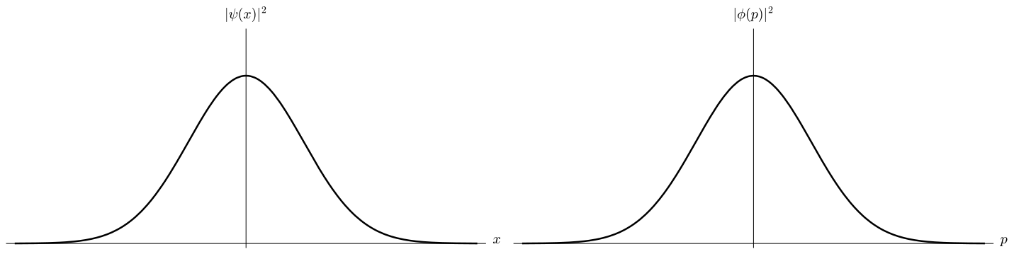
The typical situation for the probability distributions over position and wave number is illustrated below.

Using $E = \hbar\omega$ and $p=\hbar k$, and defining $\tilde{\phi}(p) = \phi(p/\hbar)/\hbar$, we can rewrite the Fourier transforms in terms of momentum as \begin{align*} \psi(x,t) & = \frac{1}{\sqrt{2\pi\hbar}} \int_{-\infty}^{+\infty} \tilde{\phi}(p) e^{i(px-E t)/\hbar}\,\mathrm{d}p, \\ \psi_0(x) & = \frac{1}{\sqrt{2\pi\hbar}} \int_{-\infty}^{+\infty} \tilde{\phi}(p) e^{ipx/\hbar}\,\mathrm{d}p, \\ \tilde{\phi}(p) & = \frac{1}{\sqrt{2\pi\hbar}} \int_{-\infty}^{+\infty} \psi_0(x) e^{-ipx/\hbar}\,\mathrm{d}x, \end{align*} and then $|\tilde{\phi}(p)|^2$ is the probability density for momentum.

Don't worry if you do not follow the details of this, as we will do these calculations in more detail in the next module.

The typical situation for a wavefunction in which both $x$ and $p$ are well-localized is illustrated below.

As an example consider the wave function \[\psi_0 = \left ( \frac{1}{2\pi\sigma^2}\right )^{\frac{1}{4}} e^{-x^2/4\sigma^2}.\] This is chosen so that the probability density for position \[|\psi_0|^2 = \frac{1}{\sqrt{2\pi\sigma^2}} e^{-x^2/2\sigma^2},\] is a Gaussian probability density with mean $0$ and standard deviation $\Delta x = \sigma$.

We can now try to compute the momentum amplitude $\tilde{\phi}(p)$ by taking the Fourier transform. \begin{align*} \tilde{\phi}(p) & = \frac{1}{\sqrt{2\pi\hbar}} \left ( \frac{1}{2\pi\sigma^2}\right )^{\frac{1}{4}} \int_{-\infty}^{+\infty} e^{-\left ( \frac{x^2}{4\sigma^2} + \frac{ipx}{\hbar} \right )}\,\mathrm{d}x & = \left ( \frac{1}{2^3\pi^3\hbar^2 \sigma^2}\right )^{\frac{1}{4}} \int_{-\infty}^{+\infty} e^{-\left ( \frac{x^2}{4\sigma^2} + \frac{ipx}{\hbar} \right )}\,\mathrm{d}x. \end{align*}

To solve this integral, we complete the square for the term in the exponential: \[\frac{x^2}{4\sigma^2} + \frac{ipx}{\hbar} = \left ( \frac{x}{2\sigma} + \frac{ip\sigma}{\hbar}\right )^2 + \frac{p^2\sigma^2}{\hbar^2},\] so we can rewrite the integral as \[\tilde{\phi}(p) = \left ( \frac{1}{2^3\pi^3\hbar^2 \sigma^2}\right )^{\frac{1}{4}} e^{-\frac{p^2 \sigma^2}{hbar^2}} \int_{-\infty}^{+\infty} e^{-\left ( \frac{x}{2\sigma} + \frac{ip\sigma}{\hbar}\right )^2 } \,\mathrm{d}x.\]

Making the substitution $y = \frac{x}{2\sigma} + \frac{ip\sigma}{\hbar}$ gives $\mathrm{d}y = \frac{\mathrm{d}x}{2\sigma}$, and \[\tilde{\phi}(p) = \left ( \frac{2\sigma^2}{\pi^3\hbar^2}\right )^{\frac{1}{4}} e^{-\frac{p^2 \sigma^2}{hbar^2}} \int_{-\infty}^{+\infty} e^{-y^2}\,\mathrm{d}y.\]

We can then use $\int_{-\infty}^{+\infty} e^{-y^2}\,\mathrm{d}y = \sqrt{\pi}$ to obtain \[\tilde{\phi}(p) = \left ( \frac{2\sigma^2}{\pi\hbar^2}\right )^{\frac{1}{4}} e^{-\frac{p^2\sigma^2}{\hbar^2}},\] from which we get the probability density \[|\tilde{\phi}(p)|^2 = \sqrt{\frac{2\sigma^2}{\pi\hbar^2}} e^{\frac{p2^2\sigma^2}{\hbar^2}}.\] This is also a Gaussian probability density, which can be written in the standard form as \[|\tilde{\phi}(p)|^2 = \sqrt{\frac{1}{2\pi \left ( \frac{\hbar}{2\sigma}\right )^2}} \exp \left ( -\frac{p^2}{2 \left ( \frac{\hbar}{2\sigma} \right )^2} \right ).\] This is a Gaussian probability density centered at $p=0$ with standard deviation $\Delta p =\frac{\hbar}{2\sigma}$.

Since $\Delta x = \sigma$, we have \[\Delta x \Delta p = \frac{\hbar}{2}.\]

This shows that Gaussian states are localized in $x$ and $p$ and are subject to minimal uncertainty with respect to the uncertainty priniple (interpreted as preparation uncertainty) so are good candidates to approximate the state of a classical particle.

This is our first rigorous demonstration of the uncertainty principle, but of course we will need to show that it holds for all wavefunctions, not just Gaussian ones.

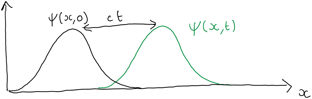
The motion of a wave packet depends on the dispersion relation $\omega(k)$ of the wave equation it satisfies, i.e. the angular frequency expressed as a function of wave number. A one dimensional system is called nondispersive if $\omega = kc$ for some constant $c$. Then, we have \[\psi(x,t) = \frac{1}{\sqrt{2\pi}} \int_{-\infty}^{+\infty} \phi(k) e^{ik(x-ct)}\,\mathrm{d}k = \psi_0(x-ct).\]

In this case, the wave packet keeps the same shape over time and just moves to the right with velocity $c$, as illustrated below.

Note that $\omega = kc$ implies $\hbar \omega = \hbar k c$, or $E = pc$, so in quantum mechanics only free massless particles, like photons, are nondispersive. In general, we will have dispersion. For example, for a nonrelativistic free massive particle we have \[E = \frac{p^2}{2m}\qquad \Rightarrow \qquad \hbar \omega = \frac{\hbar^2k^2}{2m}\qquad \Rightarrow \qquad \omega = \frac{\hbar k^2}{2m}.\]

When there is dispersion:

• The fast oscillations move at a different velocity to the overall envelope of the wave packet. The former move at the phase velocity $v_p$ and the latter at the group velocity $v_g$.
• The wave packet spreads in time: $\Delta x$ increases.

The difference between phase and group velocity is illustrated below. It is perhaps clearer to understand the difference from a video.

Note that the video shows a situation in which we have a periodic envelope with faster oscillations within it. However, the situation where the envelope is not periodic is similar. The phase velocity can be slower, the same, or faster than the group velocity depending on the dispersion relation.

The video below illustrates how a Gaussian wave packet spreads over time. This wave packet has an initial average position of zero and an initial average momentum of zero, so only the spreading effect is present. In general, the wave packet would also move to the right or left in addition to spreading.

In general, the phase and group velocities are given by \begin{align*} v_p & = \frac{\omega}{k}, & v_g & = \frac{\mathrm{d}\omega}{\mathrm{d}k}. \end{align*}

In an in-class activity, you will show that this implies that, in quantum mechanics \begin{align*} v_p = & \frac{E}{p}, & v_g & = \frac{\mathrm{d}E}{\mathrm{d}p}. \end{align*}

Now, consider a nonrelativistic system with a constant potential \[E = \frac{p^2}{2m} + V.\] Then, we have \begin{align*} v_p & = \frac{p}{2m} + \frac{V}{p}, & v_g = \frac{p}{m}. \end{align*} Since, classically, $p=mv$, it is the group velocity, not the phase velocity, that corresponds to the velocity of a classical particle. In other words, the motion of the overall envelope is classical (when the potential is constant). Note, this is another reason why plane wave solutions are not physically realizable. For a plane wave, the phase and group velocities are equal, and do not obey the classical equation $p=mv$.

Although we sometimes model a “classical” particle as a wave packet with $\Delta x, \Delta p \sim \hbar$, it is not really classical because the wave packet spreads in time.

Without going into details of the calculation, if we have an initial Gaussian wave packet \[\psi(x,0) = \left ( \frac{1}{2\pi\sigma_0^2}\right )^{\frac{1}{4}} e^{\left [ -x^2/4\sigma_0^2 + ikx \right ]},\] then, under free evolution $V = 0$, the wave packet remains Gaussian but the width increases to \[\sigma_t = \sigma_0\sqrt{1 + \frac{\hbar^2t^2}{4m^2\sigma_0^4}}.\]

1. Use \begin{align*} v_p & = \frac{\omega}{k}, & v_g & = \frac{\mathrm{d}\omega}{\mathrm{d}k}, \end{align*} together with \begin{align*} E & = \hbar \omega, & p& = \hbar k, \end{align*} to show that \begin{align*} v_p & = \frac{E}{p}, & v_g & = \frac{\mathrm{d}E}{\mathrm{d}p} \end{align*}
2. Consider a particle with initial position uncertainty $\sigma_0 = 1\,\text{nm}$. Using \[\sigma_t = \sigma_0\sqrt{1 + \frac{\hbar^2t^2}{4m^2\sigma_0^4}},\] determine how long it would take for the wave packet to have $\sigma_t = 1\,\text{m}$ if

   1. $m=9.11\times 10^{-31}\,\text{kg}$ (the mass of an electron),
   2. $m=70\,\text{kg}$ (the mass of a physics instructor).